More motivation on why we want models
We want to build models for our model-based RL algorithms because they might help us with the data-efficiency problem. Let's take a look again at the objective we want to optimize\[
\begin{equation}
\label{eq:objective}
\underset{\theta}{\operatorname{argmax}} V(\theta) = \mathbb{E}_{P(\tau|\theta)}\left\lbrace R(\tau) \right\rbrace
\end{equation}
\]
The distribution over trajectories $P(\tau| \theta)$ describes which sequences of states and actions $s_0,a_0,...,s_{H-1},a_{H-1}$ are likely to be observed when applying a policy with parameters $\theta$. Since we're working under the MDP framework, sampling trajectories $\tau$ is usualy done with the following steps:
Although this example is a bit funny, there are other cases where sampling trajectories from a real system would be too risky: controlling a power plant, launching a rocket, controlling the traffic lights in a city,... We hope that generic algorithms like RL could solve these problems one day, but we can't just let our software agent learn from trial-and-error when mistakes have considerable cost.
\[\begin{align*}s_{t+1} &= f(s_t, a_t) + \epsilon, &\epsilon \sim P(\epsilon) \\
&= f_{\mathrm{sim}}(s_t, a_t) + f_{\mathrm{data}}(s_t, a_t) + \epsilon, &\epsilon \sim P(\epsilon)
\end{align*}\] Here $\epsilon$ is independent additive noise (although there's no reason why it should be independent). $f_{\mathrm{sim}}$ represents our simulated environment, where we put out prior knowledge and $f_{\mathrm{data}}$ the corrections we apply from new data we obtain . This is just one of the many ways we could combine a simulator with a data driven model. Also, we could just use the data driven model $f_{\mathrm{data}}$ and ignore $f_{\mathrm{sim}}$. In any case, introducing the model $f$, we would apply RL algorithms with the following procedure:

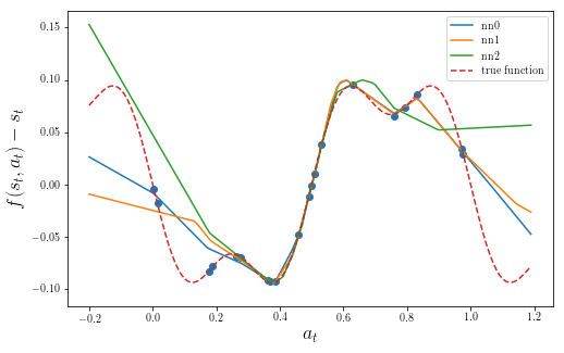
Now we try to fit a simple feed-forward neural network model. We try it three different times, with different starting conditions, and get the following predictors:

Which model should we pick for optimizing the policy? Depending on which model we decide to use, we will get different results. If we compare these models with the true underlying function, we can see that all of them a biased in regions where data is sparse.
 We could try collecting more data to improve the models, but that would only work if the data that we have collected includes information about good trajectories, i.e. the ones that maximize the objective ($\ref{eq:objective}$).
One important observation in this example is that different models make different mistakes. For example, the nn3 model is closer to the true function for $a_t < 0.5$, while the other two models are closer for $a_t > 0.5$. We refer to the fact that we don't know which of the models is a better fit for the data, unless we collect more data, as modelling uncertainty. This modelling uncertainty is reflected in the distribution of possible explanations for our data.
That is, to obtain samples from the dynamics model, we should consider all possible hypotheses for our model. This also changes the trajectory distributions that we get from applying the policy using our model as \[ \begin{equation} \label{eq:uncertain_traj} P\left(\tau \middle| \theta\right) = \int P\left(\tau \middle| \theta, M\right) P\left(M \middle| \mathcal{D}_{\mathrm{target}}\right) \mathrm{d}\mathrm{M} \end{equation} \]
Going back into our objective function $(~\ref{eq:objective})$, if we plug in the expression $(~\ref{eq:uncertain_traj})$ we will get \[ \begin{align} \label{eq:opt2} \begin{split} \underset{\theta}{\operatorname{argmax}} V(\theta) &= \int P(\tau|\theta) R(\tau) \mathrm{d}\tau \\ &= \int \int P\left(\tau \middle| \theta, M\right) P\left(M \middle| \mathcal{D}_{\mathrm{target}}\right) R(\tau) \mathrm{d}M \mathrm{d}\tau\\ &= \mathbb{E}_{P(\tau, M|\theta, \mathcal{D}_{\mathrm{target}})}\left\lbrace R(\tau) \right\rbrace \end{split} \end{align} \] With this objective, we are now trying to maximize the rewards in expectation, under the joint distribution of trajectories and models. This objective is accounting for model uncertainty since we are never sure of what are the true dynamics: we only have a belief that is dependent on the data.
As mentioned in a previous post, PILCO approximates this objective by analytical integration. The integral in ($\ref{eq:uncertain_dyn}$) is calculated analytically via the use of Gaussian Process (GP) regression model. $P(s_t)$, which is needed for evaluating the objective, is obtained by integrating over $P(s_{t-1}, a_{t-1})$, which is assumed to be Gaussian. We have use PILCO successfully for training controllers for an underwater swimming robot. However, PILCO has a high computational cost, and does not scale to large datasets or high dimensional systems (see section 2.3.4 of Marc Deisenroth's PhD thesis).
Although we could try using some of the more recent methods for scaling up Gaussian Process regression (e.g. kernel interpolation methods), we are going to focus instead on the use of Bayesian Neural Networks (BNNs). The main motivations are their widespread use, the availability of software and hardware tools, and their favorable scalability when compared with vanilla GP regression. In the next post, we'll see how to implement simpe variants of BNNs, which we will then use with a variety of RL algorithms.
The distribution over trajectories $P(\tau| \theta)$ describes which sequences of states and actions $s_0,a_0,...,s_{H-1},a_{H-1}$ are likely to be observed when applying a policy with parameters $\theta$. Since we're working under the MDP framework, sampling trajectories $\tau$ is usualy done with the following steps:
- Sample an initial state $s_0 \sim P(s_0)$
- Repeat for $H$ steps
- Evaluate policy $a_t \sim \pi_{\theta}(a_t|s_t)$
- Apply action to obtain next state $s_{t+1} \sim P(s_{t+1}|s_t, a_t)$
- Obtain reward $r_t$
 |
| Let's solve this with RL! |
Using Models for Learning
We can try writing a simulator for the system we want to control and apply policy gradients in that setting. This, of course, requires models to be accurate. This is generally not the case, and researchers in the field call this situation the reality gap: the discrepancy between simulation models and reality. The effect on RL algorithms is that a policy that has been optimized in simulation will not necessarily work in the real world. Here's a quote from a paper by Todorov, Tassa an Erez describing what is part of the issueSims [7] pointed out, if the physics engine allows cheating the optimization algorithm will find a way to exploit it – and produce a controller that achieves its goal (in the sense of optimizing the specified cost function) in a physically unrealistic way. This has been our experience as well.This is also the issue of modelling bias that I mentioned in previous posts. To fix this problem, we can try using data collected on the robot system to correct for the errors in simulation. For example, if we assume that the real system's dynamics can be modelled by a deterministic function corrupted by noise, we can model the transition dynamics as
\[\begin{align*}s_{t+1} &= f(s_t, a_t) + \epsilon, &\epsilon \sim P(\epsilon) \\
&= f_{\mathrm{sim}}(s_t, a_t) + f_{\mathrm{data}}(s_t, a_t) + \epsilon, &\epsilon \sim P(\epsilon)
\end{align*}\] Here $\epsilon$ is independent additive noise (although there's no reason why it should be independent). $f_{\mathrm{sim}}$ represents our simulated environment, where we put out prior knowledge and $f_{\mathrm{data}}$ the corrections we apply from new data we obtain . This is just one of the many ways we could combine a simulator with a data driven model. Also, we could just use the data driven model $f_{\mathrm{data}}$ and ignore $f_{\mathrm{sim}}$. In any case, introducing the model $f$, we would apply RL algorithms with the following procedure:
- Repeat for N optimization iterations
- Apply policy $\pi_{\theta}$ to collect trajectory data
- Use new trajectory data to update $f$
- Obtain new parameters $\theta$ by optimize $(\ref{eq:objective})$, simulating trajectories using $f$
Dealing with Model Bias
To illustrate the issue with bias, imagine that we have a system with one dimensional state. At time $t=0$, we can apply an action $a_0$, which changes the current state by some amount; i.e. $f(s_t, a_t) = s_t + \delta(a_t)$. The code for this example is available here. After applying random controls to the system , we might have obtained a dataset that looks like the following picture:Which model should we pick for optimizing the policy? Depending on which model we decide to use, we will get different results. If we compare these models with the true underlying function, we can see that all of them a biased in regions where data is sparse.
One important observation in this example is that different models make different mistakes. For example, the nn3 model is closer to the true function for $a_t < 0.5$, while the other two models are closer for $a_t > 0.5$. We refer to the fact that we don't know which of the models is a better fit for the data, unless we collect more data, as modelling uncertainty. This modelling uncertainty is reflected in the distribution of possible explanations for our data.
Accounting for model uncertainty
So, we could try to find a robust policy, one that works well under any model that explains our data. By taking the Bayesian approach, we may say that the data that we collect $\mathcal{D}_{\mathrm{target}}$ provides us information about the unknown model $M$: \[ \begin{equation} \label{eq:uncertain_dyn} s_t \sim P\left(s_t \middle| s_{t-1}, a_{t-1}\right) = \int P\left(s_t \middle| s_{t-1}, a_{t-1}, M\right) P\left(M \middle| \mathcal{D}_{\mathrm{target}}\right) \mathrm{d}\mathrm{M} \end{equation} \]That is, to obtain samples from the dynamics model, we should consider all possible hypotheses for our model. This also changes the trajectory distributions that we get from applying the policy using our model as \[ \begin{equation} \label{eq:uncertain_traj} P\left(\tau \middle| \theta\right) = \int P\left(\tau \middle| \theta, M\right) P\left(M \middle| \mathcal{D}_{\mathrm{target}}\right) \mathrm{d}\mathrm{M} \end{equation} \]
Going back into our objective function $(~\ref{eq:objective})$, if we plug in the expression $(~\ref{eq:uncertain_traj})$ we will get \[ \begin{align} \label{eq:opt2} \begin{split} \underset{\theta}{\operatorname{argmax}} V(\theta) &= \int P(\tau|\theta) R(\tau) \mathrm{d}\tau \\ &= \int \int P\left(\tau \middle| \theta, M\right) P\left(M \middle| \mathcal{D}_{\mathrm{target}}\right) R(\tau) \mathrm{d}M \mathrm{d}\tau\\ &= \mathbb{E}_{P(\tau, M|\theta, \mathcal{D}_{\mathrm{target}})}\left\lbrace R(\tau) \right\rbrace \end{split} \end{align} \] With this objective, we are now trying to maximize the rewards in expectation, under the joint distribution of trajectories and models. This objective is accounting for model uncertainty since we are never sure of what are the true dynamics: we only have a belief that is dependent on the data.
As mentioned in a previous post, PILCO approximates this objective by analytical integration. The integral in ($\ref{eq:uncertain_dyn}$) is calculated analytically via the use of Gaussian Process (GP) regression model. $P(s_t)$, which is needed for evaluating the objective, is obtained by integrating over $P(s_{t-1}, a_{t-1})$, which is assumed to be Gaussian. We have use PILCO successfully for training controllers for an underwater swimming robot. However, PILCO has a high computational cost, and does not scale to large datasets or high dimensional systems (see section 2.3.4 of Marc Deisenroth's PhD thesis).
Although we could try using some of the more recent methods for scaling up Gaussian Process regression (e.g. kernel interpolation methods), we are going to focus instead on the use of Bayesian Neural Networks (BNNs). The main motivations are their widespread use, the availability of software and hardware tools, and their favorable scalability when compared with vanilla GP regression. In the next post, we'll see how to implement simpe variants of BNNs, which we will then use with a variety of RL algorithms.
Comments
Post a Comment